Summary:

Path generation with obstacle avoidance was done with an energy based avoidance algorithm. This code would take in two locations for the PnP action and create a path in the XYZ space.

Theory:

The theory behind the algorithm for path planning with obstacle avoidance is rooted in the idea of attraction and repulsion. The algorithm essentially takes linear steps between point A and point B, based on the amount of attraction force there is to the target. However, if during the update step the current position in the trajectory encounters a predefined repulsion force within its range, the next position will consider this in the calculation of its next step. This next position calculation is shown in the figure below as the summation of the attraction and repulsion forces for the step.

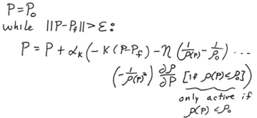
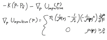
For the equation to work properly, values k, η, ρ, and α must be tuned such that there is no collision into the obstacle and so that the obstacle does not repulse too much once within the repulsion radius. k, η, ρ, and α represent the linear attraction, net repulsion, repulsion radius and step update constants respectively. The working constants for the implemented algorithm are shown in the application.

Application:

The code for this algorithm was written in python and it takes in arguments for final and desired positions. In addition, the path generation algorithm is integrated with the inverse kinematics algorithm so that for each step along the path, joint angles are also given.

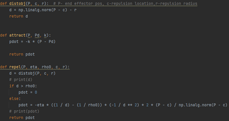
The equations for the repulsion and attraction forces from the theory section were implemented into the python code. This is shown in the figure below.

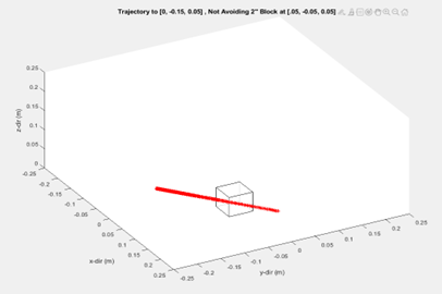
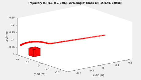
One artifact to note from the generation of paths using this method is that due to using forces and updates, the distance between points along the path are not constant. The density of points increases when the path is in the repulsion field. To account for this in the creation of a smooth motion for the robot, the norm between the joint angles is taken and then multiplied by a factor so that we can create a constant time between positions and thus a constant velocity throughout the path. Paths were then simulated in MatLab to show the algorithm working. A comparison between the path generation with and without avoidance was done and shown in the figures below.